Currently migrating my blog from wordpress and other scattered sources.
Estimating the crack
This is a simple method to quatitatively estimate crack on a damaged phone screen. Mapping an image to a numerical quantity using basic image processing is the generic problem addressed. Sample images of cracked screen are approx 160 X 250 pixels and the repo can be found here.
Major Processing Steps:
Preprocessing image » Scan with a sliding window » Estimate Crack %
Preprocessing
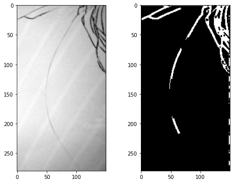
- Convert to grascale image
- Use canny edge detection to identify the cracks. The result is a binary image with
1s where the cracks are detected and0s elsewhere.
# importing necessary libraries
import numpy as np
from skimage.color import rgb2gray
from skimage.io import imread
from skimage import feature, img_as_bool
from skimage.morphology import binary_dilation, binary_erosion
import matplotlib.pyplot as plt
url = "./data/crack_1.png"
img1 = imread(url)

def preprocess(url):
    img = imread(url)
    img = rgb2gray(img)
    img_edge = binary_erosion(binary_dilation(feature.canny(img, sigma =.1)))
    return img, img_edge
fig = plt.figure(figsize = (8,6))

img1,c1 = preprocess(url)

ax1 = fig.add_subplot(121)
plt.imshow(img1, cmap='gray')
ax2 = fig.add_subplot(122)
plt.imshow(c1, cmap='gray')

plt.show()
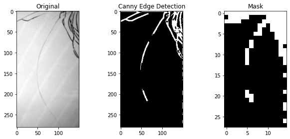
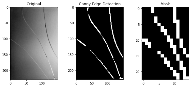
Scanning with sliding window
-
A non-overlapping sliding window of size
10 X 10is used to scan through the image. Each instance of the sliding window returns a label1or0based on the fraction of white pixels (crack density) present in that window. The threshold (varies from 0 to 1) for this classification can be adjusted for strict or lax classification. The sliding window allows us to draw a bounding box encompassing the crack inside. -
The labels of the
ith row andjth column of scanning window is aggregated using the binary matrix A(i,j). An image representation of this matrix is shown alongside processed images (as Mask).
Estimate Crack %
- The crack % is estimated as the fraction of
1labels compared to the total elements in the matrix.
def edge_prob(window, cut_off):
    pixels  = np.array(window.ravel())
    if ((np.count_nonzero(pixels)/len(pixels))>cut_off):
        return 1
    else:
        return 0

def sliding_mat(img,window_x=10,window_y=10, cut_off=0.1):

    arr_x = np.arange(0,img.shape[0],window_x)
    arr_y = np.arange(0,img.shape[1],window_y)

    A = np.zeros((len(arr_x),len(arr_y)))

    for i,x in enumerate(arr_x):
        for j,y in enumerate(arr_y):
            window = img[x:x+window_x,y:y+window_y]
            A[i,j] = edge_prob(window, cut_off=cut_off)

    return A, arr_x, arr_y

def plot_all(img,canny_edge,A):
    fig = plt.figure(figsize = (9,4))
    ax1 = fig.add_subplot(131)
    ax1.imshow(img, cmap="gray")
    ax1.set_title("Original")

    ax2 = fig.add_subplot(132)
    ax2.set_title("Canny Edge Detection")
    ax2.imshow(canny_edge, cmap="gray")

    ax3 = fig.add_subplot(133)
    ax3.set_title("Mask")
    ax3.imshow(A,cmap="gray")
    plt.tight_layout()
    plt.show()

A, arr_x, arr_y = sliding_mat(c1, window_x=10, window_y=10, cut_off=0.1)

print("Estimate of crack : {:.2f}%".format(np.sum(A)/A.size*100))
plot_all(img1,c1,A)
Estimate of crack : 18.57%
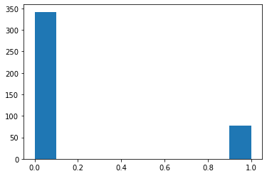
print("Shape of image {}\nShape of : A {}".format(c1.shape,A.shape))
plt.hist(A.ravel())
plt.show()
Shape of image (280, 150)
Shape of : A (28, 15)
Test Cases
#2 Low Crack
url_2 = "./data/crack_2.png"
img2,c2 = preprocess(url_2)
A, arr_x, arr_y = sliding_mat(c2,window_x=10, window_y=10, cut_off=0.1)

print("Estimate of crack : {:.2f}%".format(np.sum(A)/A.size*100))
plot_all(img2,c2,A)
Estimate of crack : 17.39%
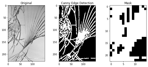
#3 High Crack
url_2 = "./data/crack_3.png"
img2,c2 = preprocess(url_2)
A, arr_x, arr_y = sliding_mat(c2,window_x=10, window_y=10, cut_off=0.1)

print("Estimate of crack : {:.2f}%".format(np.sum(A)/A.size*100))
plot_all(img2,c2,A)
Estimate of crack : 72.46%
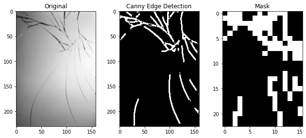
#4 Medium Crack
url_2 = "./data/crack_4.png"
img2,c2 = preprocess(url_2)
A, arr_x, arr_y = sliding_mat(c2,window_x=10,window_y=10, cut_off=0.1)

print("Estimate of crack : {:.2f}%".format(np.sum(A)/A.size*100))
plot_all(img2,c2,A)
Estimate of crack : 26.63%
Perspective
This method can be used to create a labeled dataset mapping image=>labels to be trained on an algorithm. For example after we map phone_1 => crack_1 %, we may take multuple images at various different angles for that particular phone i.e phone_1 while mapping all of them to the same crack_1 %. By aggregating images from different phone models, we can create a reliable dataset for advanced modelling techniques such as neural networks.