Error measures to Understand Forecast Quality

Aim of any forecasting system is to improve the decision-making framework through predictions using past i.e. data. Although, for many practical purposes like reporting we use a single-valued point forecast, there are scenarios where prediction intervals from probabilistic forecasts can aid decision making by calculating associated risk.

In describing the quality of forecast accuracy, error and loss are some general metrics that are often quoted to choose between two competing forecasting models. Errors can be monitored at two levels a) business metrics b) model performance. It is imperative to monitor both these metrics to track the change for every cycle of predictions to understand the drift (or depletion of forecast quality). A substantial change in any of the metrics should be investigated as it might lead to the nature of model’s [mis]behaviour.

Here, I discuss various metrics which can be used “together” to avoid the pitfalls related to optimizing a single metric. Following a single metric alone can be misleading when it comes to the quality of forecast as it might be practically useless despite the stellar performance of that particular metric. It is practically impossible to reduce all error metrics to only one dimension without sacrificing information since each metric gives us complementary information about the forecast.

For us, the important question at hand is to decide between two competing forecasts based on the error. The issue gets accented when quantifying the quality of thousands of time-series predicted in one shot as it limits our ability to check each one individually. Hence, we resort to aggregate error statistics. Ideally, a replacing forecasting system with reliable predictions should improve all error metrics w.r.t existing benchmark. Moreover, the replacing system should ultimately serve the goals of the organization whatever the metrics be.

Point Forecast

Most of these metrics are drawn from user manual of M5 competition.

MAPE + BIAS + absolute_error

MAPE(Mean Absolute Percentage Error) is the most identifiable and often quoted business metric. In this implementation, tolerance is used to avoid NaNs.

import numpy as np

def mape_and_bias(true, predict, tol=1e-10):
    error = predict-true
    bias = error/(true+tol)
    abs_error = np.abs(error)
    mape = abs_error/(np.abs(true)+tol)
    return mape, bias, abs_error # for caped mape: min(mape,1)

Weighted MAPE or wMAPE

A single weighted value for MAPE is required when comparing two different algorithms/forecasting systems invovling multiple timeseries. For example if there are 100 timeseries, sum of weighted MAPE is calculated as $wMAPE = \sum_{i=1}^{100}w_{i}\times MAPE_{i}$. Another non-dimensional measure can be calculated as $ND = \frac{\sum_{i}forecast_{i}}{\sum_{i}actuals_{i}}$

Symmetric MAPE or sMAPE

Symmetric MAPE is a useful metric when actuals/predictions are close to 0. sMAPE addresses the situation of exploding error metric through division when denominator $ \rightarrow 0 $. A weighted value can be calulated as in the case of wMAPE as well.

def smape(true, predict, tol=1e-10):
    denominator = np.abs(target) + np.abs(forecast) + tol
    return 2*np.abs(target - forecast) / denominator

RMSE and Normalized RMSE

RMSE a.k.a Root Mean Squared Error is the L2 version of MAPE, and it can be normalized by absolute error to get a normalized value nRMSE.

def rmse_and_nrmse(true, predict):
    error = predict-true
    rmse = np.mean(np.sqrt(error^2))
    abs_error = np.mean(np.abs(error))
    nrmse=rmse/abs_error
    return rmse, nrmse

MASE - Mean Absolute Scaled Error

MASE will calculate the value-add of a forecasting system by comparing to a naive forecast i.e a forecast from the training example. This is a relative measure of our forecasting system w.r.t a naive estimate.

def mase(true, predict, naive_forecast):
    return np.mean(np.abs(true - predict)) / np.mean(np.abs(true - naive_forecast))

OWA - Overall Weighted Average

This is a metric popularized by M-competitions to rank the competitors. Here a naive forecast is created by taking the median value from the past season, i.e. for a naive forecast of Jan 2020, we can take the median value of Jan-2019, Jan-2018 etc. All error metrics mentioned can be calculated w.r.t actuals from the naive forecast to create a naive estimate.

Probabilistic Forecast

There are some instances where some key decisions are made based on the uncertainty in the forecast and it is vital to assess forecast quality using prediction intervals from distribution rather than point estimates. I aim to create a reasonable intuition on interpreting these metrics. All the errors discussed in the point forecasts can be calculated for probabilistic forecasts by choosing a midpoint such as the median or the mean.

Quantile Loss and Coverage

Quantiles divide a probability distribution into regions of equal probability. Although named as quantile loss, the function can measure the deviation of each predicted percentile (thereby learning the whole distribution) from the target by passing the percentile as a parameter q to loss function. Quantile loss should be seen in the context of Coverage which gives the proportion of predictions north of actualsand helps us estimating whether each percentile is under/over forecasting. Given a more accurate predicted distribution, higher percentile should give higher coverage as they give a higher expectation than the median and vice versa.

## coverage
def coverage(target, forecast):
    return (np.mean((target < forecast)))

## quantile loss
def quantile_loss(target, forecast, q):
    return (2*np.sum(np.abs((forecast-target)*((target<=forecast)-q))))

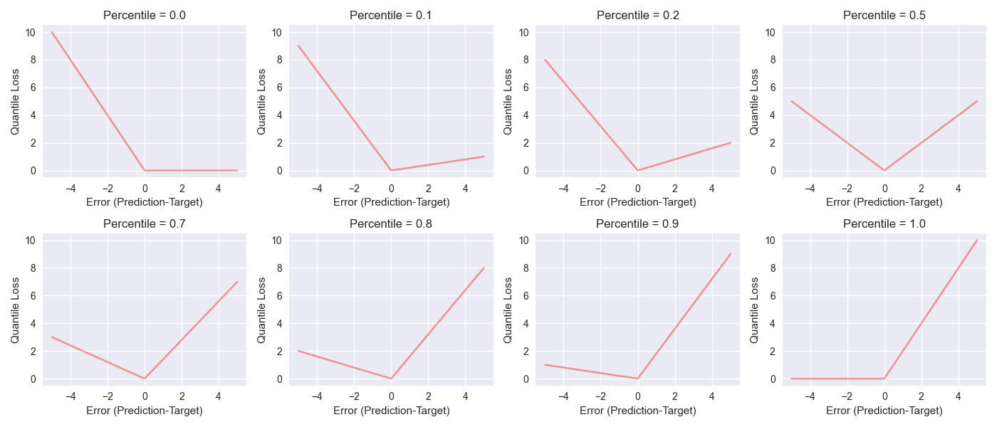
The figure below will help us understand the difference in weighting on error for loss calculation. They are generted using quantile_loss. Particularly we should look at the difference in weighting for positive and negative error for a given percentile. For percentile q==0.5, weigthing in loss function equally penalize both positive and negative errors. For the lowest percentile q==0.0 loss function ignores positive error, the quantile loss make sure that the predicted 0.0^th percentile is the lowest expectation. Depending on the percentile, the positive and negative error is weighted differently. The multiplication by 2 in quantile_loss is a convenience which ensures the return of a magnitude of 2 x 0.5 x abs(forecast-target) for q==0.5.

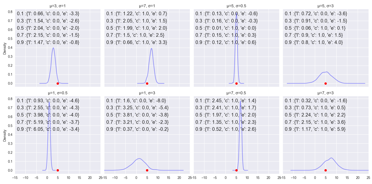
Given a target value(=5 as red dot) and a predicted distribution( blue), the plots below gives an intuition of quantile-loss “l”, coverage “c” and error “e”=(prediction-target) for percentiles=[0.1,0.3,0.5,0.7,0.9].

weighted loss

Weighted Quantile loss for a given quantile q is calculated with division by sum of absolute target, i.e. absolute sum of the target.

MSIS - Mean Scaled Interval Score

Simillar to MASE, MSIS compares the forecast error to a baseline seasonal_error calculated from naive forecast.

def msis(target,lower_quantile,upper_quantile,seasonal_error,alpha):
    """alpha - significance level"""
        numerator = np.mean(
            upper_quantile-lower_quantile
            + 2.0/ alpha* (lower_quantile - target)*(target < lower_quantile)
            + 2.0/ alpha*(target - upper_quantile)*(target > upper_quantile)
        )
        return (numerator/seasonal_error)

Conclusion

With all things mentioned above, a refined forecasting system must reflect the distinct costs associated with underprediction and overprediction. For example, over-forecasting is costly when a factory produce an item(like drugs) with a short expiry date since we may have lesser opportunities to sell it leading to wastage. In such cases, we need to approach the target from below and under-forecasting has to be favored. On the other hand, over-forecasting is favorable for certain generic products which are stable for a longer duration. Such items can be produced without disruption and stocked-up if inventory cost is reasonable, thus giving us more opportunities to sell them in the market without having to wait for manufacturing. The degree of tuning this bias in either direction depends on the organization, inventory capacity, economic climate, and other factors. Due to such dynamic pressures, it is challenging to maintain a good forecasting system without constant oversight.

References

1. M4 Competition
2. Hyndman Textbook